Embeddings Clustering
I explored how embeddings cluster by visualizing LLM-generated words across different categories. The visualizations helped build intuition about how these embeddings relate to each other in vector space. Most of the code was generated using Sonnet.
!pip install --upgrade pip!pip install openai!pip install matplotlib!pip install scikit-learn!pip install pandas!pip install plotly!pip install "nbformat>=4.2.0"We start by setting up functions to call ollama locally to generate embeddings and words for several categories.
The generate_words function occasionally doesn’t adhere to instructions, but the end results are largely unaffected.
from openai import OpenAI
client = OpenAI(base_url='http://localhost:11434/v1', api_key='ollama')
def get_embedding(text):
    response = client.embeddings.create(        model="nomic-embed-text",        input=text    )
    return response.data[0].embedding
def generate_words(category, num_words=25): prompt = f""" Generate {num_words} words that belong to the category '{category}'. Provide them as a comma-separated list. Output the only words now: """
response = client.chat.completions.create( model="llama3.2", messages=[ {"role": "user", "content": prompt} ], temperature=0.7, max_tokens=100 )
if response.choices[0].message and response.choices[0].message.content: words = response.choices[0].message.content.split(",") return [word.strip().lower() for word in words] return []from sklearn.manifold import TSNEimport matplotlib.pyplot as pltimport numpy as npNow we call the functions to actually generate the words and their embeddings.
category_names = [    'fruits', 'vehicles', 'sports', 'countries', 'jobs',    'weather', 'emotions', 'colors', 'furniture', 'animals',    'religions', 'verbs', 'adjectives', 'articles', 'ideologies',    'chemical_elements', 'musical_instruments', 'body_parts',    'geological_formations', 'programming_languages',    'mythological_creatures', 'diseases', 'astronomical_objects',    'mathematical_concepts', 'cooking_techniques']
categories = {name: generate_words(name, 25) for name in category_names}
strings = []labels = []embeddings = []
for category, words in categories.items():    for word in words:        strings.append(word)        labels.append(category)        embeddings.append(get_embedding(word))
Here are the first few sets of words:
for category in list(categories.keys())[:3]: print(f"\n{category.upper()}:") print(", ".join(categories[category]))print("\n...")FRUITS:apple, banana, mango, orange, grapes, watermelon, pineapple, strawberry, cherry, lemon, peach, kiwi, blueberry, pears, apricot, plum, guava, papaya, cantaloupe, raspberry, blackberry, fig, acai berry, starfruit, pomegranate, avocado
VEHICLES:car, truck, bus, train, motorcycle, bicycle, airplane, helicopter, ship, boat, ferry, ambulance, fire engine, police car, semi-truck, tractor, scooter, taxi, limousine, rv, van, buses, motorcycles, cycles, cars, vehicles, automobile
SPORTS:basketball, football, tennis, baseball, hockey, golf, rugby, cricket, boxing, wrestling, volleyball, softball, table tennis, cycling, rowing, swimming, gymnastics, skiing, snowboarding, surfing, diving, sailing, fencing, karate, lacrosse
...From here, we can visualize a 3D scatter plot of the embeddings from multiple angles.
from sklearn.decomposition import PCA
labels = []for category in category_names:    labels.extend([category] * len(categories[category]))
colors = plt.cm.tab20(np.linspace(0, 1, len(set(labels))))color_dict = dict(zip(set(labels), colors))
pca = PCA(n_components=3)pca_result = pca.fit_transform(embeddings)
fig = plt.figure(figsize=(15, 15))angles = [(45, 45), (0, 0), (90, 0), (0, 90)]titles = ['Isometric View', 'Front View', 'Side View', 'Top View']
for i, (elev, azim) in enumerate(angles, 1):    ax = fig.add_subplot(2, 2, i, projection='3d')    ax.view_init(elev=elev, azim=azim)
    colors = plt.cm.tab20(np.linspace(0, 1, len(set(labels))))    color_dict = dict(zip(set(labels), colors))
    for category in set(labels):        mask = [l == category for l in labels]        ax.scatter(pca_result[mask, 0], pca_result[mask, 1], pca_result[mask, 2],                   c=[color_dict[category]], label=category, alpha=0.6)
    ax.set_title(f'{titles[i-1]} (elev={elev}°, azim={azim}°)')
plt.legend(bbox_to_anchor=(1.05, 1), loc='upper left')plt.suptitle('3D PCA Visualization of Word Embeddings by Category')plt.tight_layout()plt.show()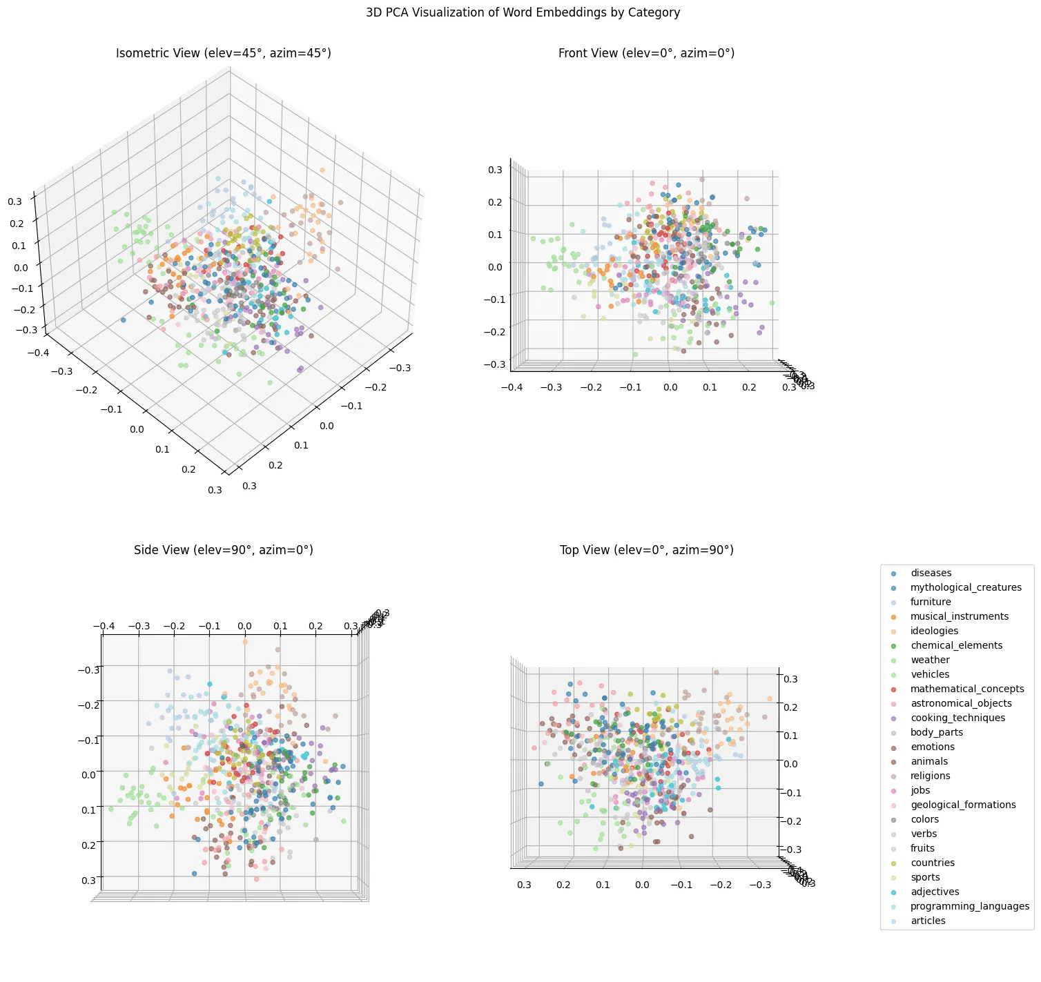
We can definitely see some clustering, but it’s a bit of a mess.
The next cell uses plotly to create an interactive visualization, where the visibility of the categories can be toggled.
Mouse over shows the word and category.
The visualization also supports rotation and panning.
I’ve included a screenshot because I haven’t found a good way to include the interactive visualization on my site yet.
import plotly.express as pximport plotly.graph_objects as goimport plotly.colors
fig = go.Figure()
colors = px.colors.qualitative.Set3[:len(set(category_names))]
n = len(category_names)colors = plotly.colors.sample_colorscale('turbo', n)color_dict = dict(zip(category_names, colors))
for category in set(labels):    mask = [l == category for l in labels]    category_words = [word for word, l in zip(strings, labels) if l == category]
    fig.add_trace(go.Scatter3d(        x=pca_result[mask, 0],        y=pca_result[mask, 1],        z=pca_result[mask, 2],        mode='markers',        name=category,        hovertext=category_words,        marker=dict(            size=6,            color=color_dict[category],            opacity=0.7        )    ))
fig.update_layout(    title='Interactive 3D PCA Visualization of Word Embeddings',    scene=dict(        xaxis_title='PC1',        yaxis_title='PC2',        zaxis_title='PC3'    ),    width=1200,    height=800,    showlegend=True,    legend=dict(        yanchor="top",        y=0.99,        xanchor="left",        x=1.05    ))
fig.show()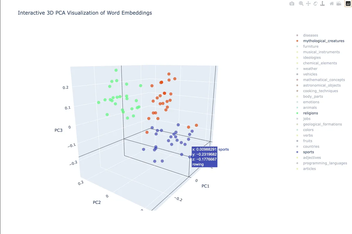
Recommended
Fine-tuning gpt-3.5-turbo to learn to play "Connections"
I started playing the NYTimes word game "Connections" recently, by the recommendation of a few friends. It has the type of freshness that Wordle lost...
Embeddings with sqlite-vector
About a year and a half ago I wrote about using sqlite-vss to store and query embedding vectors in a SQLite database. Much has changed since then and...
Practical Deep Learning, Lesson 5, Pricing Iowa Houses with Random Forests
Having completed lesson 5 of the FastAI course, I prompted Claude to give me some good datasets upon which to train a random forest model. This...